en · hplc method development ·Aug 16, 2026

HPLC Method Development: A Practical Workflow for Scientists

The fastest path to a validatable HPLC method runs through five stages: define an Analytical Target Profile (ATP), scout columns and mobile phases, optimize selectivity and system parameters, stress-test robustness, and validate against ICH Q2 criteria. For most small-molecule assays, start with a fast isocratic template if you have three or fewer analytes with similar polarity, or a generic 10-minute gradient if you’re screening a multi-component mixture without much prior data.

You can start today with three actions:

Write a one-paragraph ATP that states intended use, matrix, required limit of quantitation (LOQ), and which peak pairs absolutely must resolve.
Run a column screen across three to four complementary stationary phases under identical mobile-phase conditions.
Fire two short gradient scouting runs (different gradient times, same mobile phases) to see how peak spacing shifts before you touch anything else.

That sequence, method scouting, optimization, robustness testing, and formal validation, reflects the standard Analytical Quality by Design (AQbD) lifecycle that most modern HPLC guidance now builds around. Skip the ATP step and you’ll spend weeks chasing a separation that was never going to meet its real acceptance criteria in the first place.

Key Takeaways

A validated HPLC method comes from defining the ATP first, screening columns before tweaking solvents, and testing robustness against ICH Q2 criteria before calling any method finished.

Point	Details
Write the ATP before touching the instrument	Define intended use, matrix, required LOQ, and critical pairs before any bench work starts.
Screen columns before mobile-phase tweaks	Column chemistry drives selectivity more than solvent changes, so test stationary phases first.
Start from a template	Use a fast isocratic, generic gradient, or stability-indicating gradient as your baseline condition.
Validate against ICH Q2	Confirm accuracy, precision, specificity, LOD/LOQ, linearity, range, and robustness before transfer.
Consider automation only after a defined objective	Bayesian optimization tools help once you have a clear ATP and measurable acceptance criteria.

Why Defining the Analytical Target Profile Comes First
How Do You Scout an HPLC Method Efficiently?
Optimizing Selectivity Without Wasting Runs
Building Robustness Into a Method Before You Validate It
Fixing the Most Common HPLC Problems Fast
Copy-Paste Starting Conditions for Three Method Types
Can Automation Speed Up HPLC Method Development?
What I’ve Learned From Watching Labs Rush Method Development
Sources

Why Defining the Analytical Target Profile Comes First

An ATP is not paperwork. It’s the document that tells you which columns, mobile phases, and detectors are even worth trying, before you burn a single vial of sample.

A working ATP needs four things: the method’s intended use (identity, assay, or impurity profiling), the sample matrix and any interfering excipients or degradants, the required accuracy, precision, and LOQ, and a list of critical peak pairs that must separate with a defined resolution. Skipping any one of these turns method development into guesswork disguised as science.

Resource and risk constraints belong in the same document. Note which detectors you actually have access to (UV, PDA, mass spectrometry), your column inventory, the maximum acceptable run time for routine throughput, and how many samples per day the method needs to handle. A method that delivers baseline resolution in 45 minutes is worthless if your lab needs to process 200 samples a day.

The ATP narrows your choices immediately. If your analyte is a weak base with a pKa near 8, you already know you need a mobile phase pH well below that value to keep the compound protonated and retained on reversed-phase silica. If your intended use is a stability-indicating assay, you already know isocratic won’t cut it once degradants with different polarities show up.

Pro Tip: Before your first instrument run, build a one-page table with each analyte’s pKa, logP, UV chromophore, and expected degradation pathway. That single document routinely eliminates half of the wrong-column mistakes labs make in week one.

How Do You Scout an HPLC Method Efficiently?

Scouting is where most labs waste the most time, usually by running one column after another with essentially the same mobile phase instead of isolating variables systematically.

Start at the desk, not the bench. Check the literature for related methods, pull together your pKa and logP table, and estimate which retention mode fits: reversed-phase for most small molecules, HILIC for very polar or ionic species, ion-pairing for compounds that resist reversed-phase retention. This desk work, reviewing chemistry before touching an instrument, is what separates efficient chromatographers from those who treat the HPLC as a trial-and-error machine.

Sample preparation deserves equal attention. Dissolve your sample in the starting mobile phase or a diluent with a higher water content than your injection solvent; this single choice dramatically improves peak focusing for early-eluting compounds and prevents the split or fronted peaks that plague poorly matched diluents, according to practical HPLC guidance. Filter through a 0.22 or 0.45 micron membrane compatible with your matrix, and if the sample contains proteins, lipids, or particulates, plan a cleanup step (solid-phase extraction or protein precipitation) before it ever reaches the column.

Run two scouting gradients with different run times but identical mobile phases. This isolates the column’s inherent selectivity from gradient-driven effects and gives you a fast read on whether your critical pairs have any chance of separating.

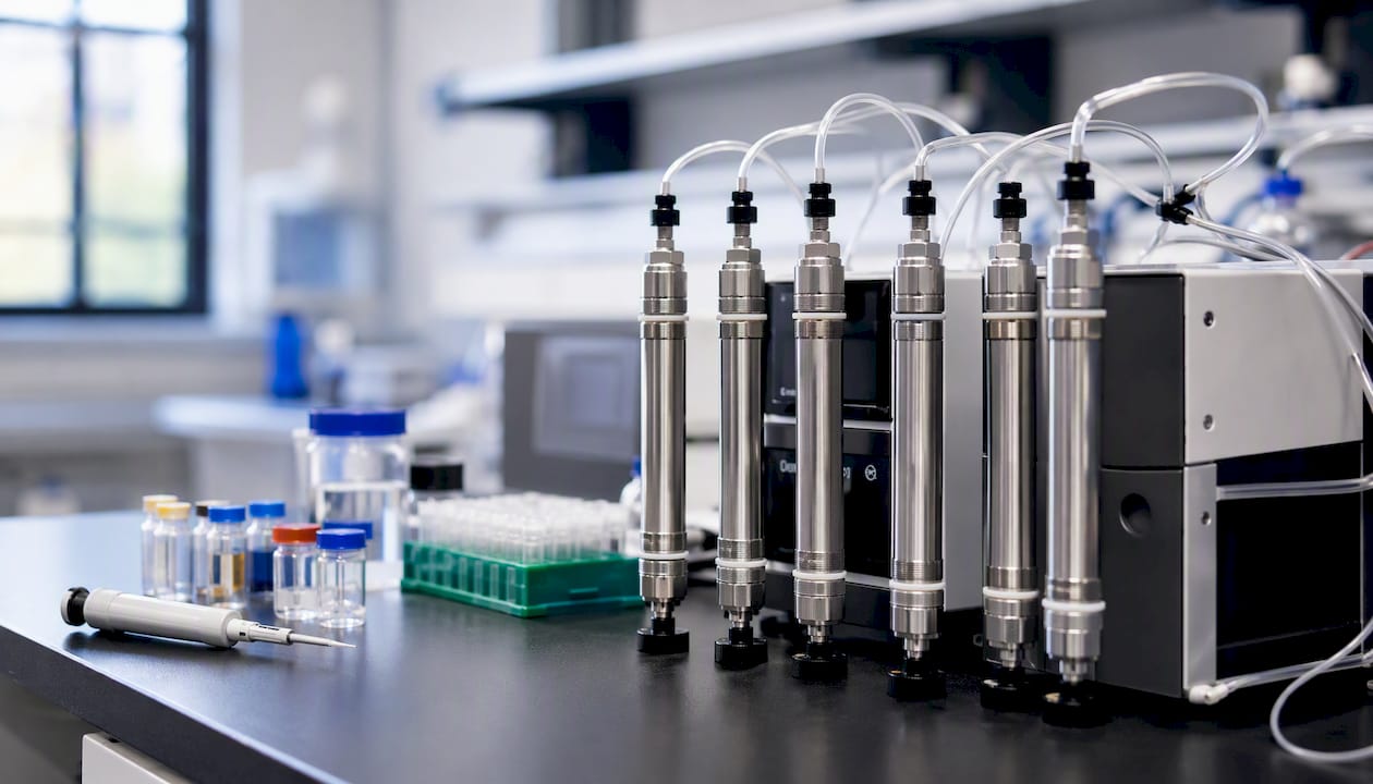
Column screening is the real lever here. Screening several stationary phases side-by-side under identical mobile-phase conditions is far more efficient than trying to rescue a poorly selected column through endless mobile-phase tweaking, since selectivity is controlled primarily by column chemistry rather than solvent composition. Method-development kits that bundle complementary phases let you hold the mobile phase constant and attribute any difference in retention or resolution directly to the stationary phase. This design detail is confirmed in Avantor’s streamlined method-development guidance.

Multiple HPLC columns side-by-side on lab bench

Analyte class	Suggested starting column	Detector mode
Neutral hydrophobic small molecules	C18, 100–150mm, 3–5μm	UV at chromophore max
Weak acids/bases	C18 with embedded polar group or phenyl-hexyl	PDA scan for peak purity
Polar/ionic compounds	HILIC or C18 with ion-pairing reagent	UV or MS, depending on ionization
Peptides and larger biomolecules	Wide-pore C18, 4.6mm	UV or MS

After scouting, run a quick system suitability check: theoretical plates, tailing factor, and resolution on your critical pair. If those numbers are already close to your targets, you’ve found your starting point. If not, you have real data to guide the next round instead of another blind guess.

Optimizing Selectivity Without Wasting Runs

Once scouting narrows your column choice, optimization is about deciding which lever to pull next, and in what order.

Column chemistry is still your strongest selectivity lever, so exhaust that option before touching anything else. Only after you’ve settled on a stationary phase should you move to the organic modifier (acetonitrile versus methanol changes selectivity, not just speed), then mobile-phase pH, then additives like ion-pairing reagents or buffer counter-ions. Changing four variables at once tells you nothing about which one mattered.

A practical optimization sequence looks like this:

Confirm column choice is final based on scouting resolution and peak shape data.
Test organic modifier type (acetonitrile vs. methanol) at a fixed pH and gradient slope.
Vary mobile-phase pH in 0.5-unit steps around your analyte’s pKa to fine-tune ionization state.
Introduce additives only if resolution of critical pairs still falls short.
Move to design of experiments (DoE) once you’ve narrowed to two or three interacting variables that single-factor testing can’t fully explain.

Single-factor testing works well for obvious, independent variables. DoE earns its keep when factors interact, when pH and temperature both shift retention of a critical pair in ways that aren’t additive, for instance. A factorial or central composite design lets you map that interaction with a defined number of runs instead of an open-ended series of guesses.

Approach	Best for	Trade-off
One-factor-at-a-time	Independent variables, early scouting, quick fixes	Misses interaction effects between factors
Design of experiments (DoE)	Multiple interacting variables, final optimization, robustness mapping	Requires more upfront planning and software

Three templates cover most early-phase work: a fast isocratic method for simple, well-characterized mixtures; a generic gradient for multi-component screening when you don’t yet know how many peaks you’re dealing with; and a stability-indicating multi-segment gradient for related-substance and degradation work where impurities span a wide polarity range. Standardized templates like these shorten early development by giving you a proven starting point instead of building a method from nothing.

Pro Tip: Run your scouting gradients overnight and log every parameter, column lot, mobile-phase batch, ambient temperature, in a shared method log. Six months from now, when a colleague tries to transfer the method, that log is the difference between a smooth handoff and a week of confused emails.

Building Robustness Into a Method Before You Validate It

A method that only works on the day you developed it isn’t a method, it’s a demonstration. Robustness testing is what turns a working separation into something you can hand to another analyst, another lab, or a regulatory reviewer with confidence.

ICH Q2 lays out the validation characteristics you need to address: accuracy, precision (repeatability and intermediate precision), specificity, limit of detection (LOD), limit of quantitation (LOQ), linearity, range, and robustness, along with solution stability where relevant. This staged approach from initial system selection through validation is what regulatory reviewers expect to see documented, not just asserted.

Robustness testing means deliberately varying the small operational parameters that change every day in a real lab, not just once during development, and confirming the method still meets its acceptance criteria.

Parameter	Typical variation range	What you’re checking
Flow rate	±0.1 mL/min	Resolution and retention time shift
Column temperature	±2 to 5°C	Selectivity and peak shape stability
Mobile-phase pH	±0.1 units	Ionization-driven retention changes
Column lot/supplier	Different lot, same specification	Batch-to-batch stationary-phase variability
Organic modifier percentage	±1 to 2%	Retention time and resolution sensitivity

Before any routine run, confirm system suitability. Commonly used targets include a tailing factor at or below 2 (ideally under 1.5), theoretical plates above 2,000, resolution of 1.5 or better between critical pairs, and percent relative standard deviation (%RSD) at or below 2% across replicate injections, benchmarks widely cited in method-development literature. These aren’t arbitrary numbers. They’re the minimum bar a method needs to clear before you trust its output.

Forced degradation studies establish that your method is genuinely stability-indicating, meaning it can distinguish the intact analyte from its breakdown products. Expose the drug substance to heat, light, acid, base, and oxidative stress, then confirm the method separates every degradant from the parent peak with acceptable resolution and mass balance. If a degradant co-elutes with your main peak, you don’t have a stability-indicating method yet, no matter how clean the chromatogram looks under normal conditions.

Documentation is what makes any of this transferable. Record acceptance criteria for every validation characteristic, the actual data generated against those criteria, instrument and column details down to the lot number, and a clear statement of the method’s intended scope. A validation package another analyst can’t reproduce from the paperwork alone isn’t finished.

Pro Tip: Build your robustness matrix as a table before you run a single sample, listing every parameter, its nominal value, and its tested range. Reviewers and future analysts read that table faster than they’ll ever read your narrative summary.

Fixing the Most Common HPLC Problems Fast

Most chromatographic problems trace back to a short list of root causes, and recognizing the pattern saves you from re-developing a method that just needs a small fix.

Common failure modes include peak tailing or fronting, low sensitivity that buries small peaks in baseline noise, co-elution of critical pairs, retention times that drift run to run, rising backpressure, and a noisy or wandering baseline.

Peak tailing: usually silanol interaction with basic analytes; try a base-deactivated column, adjust mobile-phase pH away from the analyte’s pKa, or add a small amount of triethylamine as a silanol-blocking additive.
Peak fronting: often column overload; reduce injection volume or sample concentration before assuming a chemistry problem.
Low sensitivity: check detector wavelength against the analyte’s actual UV maximum, increase injection volume if column capacity allows, or switch to a more sensitive detection mode.
Co-elution: revisit column chemistry first (see optimization above) before adjusting gradient slope, since a mismatched stationary phase rarely responds to solvent tweaks alone.
Drifting retention time: check mobile-phase pH stability, column equilibration time, and whether buffer solutions have aged past their usable window.
Rising backpressure: inspect the inline filter and guard column first; a clogged frit is the most common and most overlooked cause.
Noisy baseline: check mobile-phase purity, degas thoroughly, and confirm the detector lamp isn’t near end of life.

Before every analytical run, a short pre-run checklist prevents most of these failures: confirm mobile-phase pH and filtration, check column temperature has stabilized, verify baseline noise is within normal range, and run a system suitability sample before committing real samples to the sequence.

Pro Tip: If an early-eluting peak looks broad or split, the injection solvent is almost always the culprit before the column is. Switch to a diluent that matches or is weaker than your starting mobile phase, and that peak often sharpens up without any change to the method itself.

Copy-Paste Starting Conditions for Three Method Types

Having a reliable starting point beats building from a blank instrument method every time. These three templates cover the situations most labs encounter repeatedly.

Template A: Fast isocratic — for simple assays with two to four well-characterized analytes. Run time under 5 minutes.

Template B: Generic 10-minute gradient — for multi-component screening when peak count is uncertain. Use a 100 x 4.6mm C18 column, 3.5μm particle size, mobile phase A of 0.1% formic acid in water and mobile phase B of acetonitrile, gradient from 5% to 95% B over 8 minutes with a 2-minute hold, flow rate 1.0 mL/min, column temperature 40°C, PDA detection scanning 200 to 400nm. Gradient methods handle complex, multi-component samples better than isocratic runs because peak width stays more consistent across the whole run, though isocratic remains the more efficient choice for simpler separations.

Template C: Stability-indicating multi-segment gradient — for related-substance and degradation work. Use a 150 x 4.6mm C18 column, 3μm particle size, mobile phase A of 10mM ammonium acetate buffer at pH 4.5 and mobile phase B of acetonitrile, multi-segment gradient starting at 5% B, ramping to 40% B over 15 minutes, then to 90% B over 5 minutes to elute strongly retained impurities, flow rate 1.0 mL/min, column temperature 35°C, PDA detection with peak purity confirmation.

Adapt each template to your analyte’s chemistry before running it. A compound with a pKa near your buffer’s pH needs the buffer shifted at least one full pH unit away to avoid retention instability; a highly lipophilic analyte (logP above 4) usually needs a higher starting organic percentage to elute within a reasonable time.

Run order matters as much as the method itself. Equilibrate the column for at least 10 column volumes before the first injection, run a blank to check for carryover, then a system suitability standard, before touching real samples. Skipping equilibration is one of the most common causes of an unreproducible first injection.

Pro Tip: Name every method file with a consistent convention, analyte, column type, gradient type, and version number, so a colleague can identify what a method does without opening the instrument software. This alone cuts method-transfer confusion dramatically.

Can Automation Speed Up HPLC Method Development?

Closed-loop, operator-free optimization is moving from research curiosity to a genuinely usable tool for labs with the right infrastructure, though it’s not a replacement for the ATP and scouting work described above.

These systems use Bayesian optimization algorithms to iteratively propose experimental conditions, run them, evaluate the resulting chromatogram against defined objectives (number of resolved peaks, resolution of critical pairs, total run time), and propose the next experiment based on what it learned. Multi-objective algorithms like TS-EMO can optimize several chromatogram quality metrics simultaneously, mapping trade-offs between resolution and speed rather than chasing a single number.

A lab piloting this approach needs a short checklist in place: instrument control software capable of automated method queuing, scripts or macros to parse chromatogram data automatically, a clearly defined objective function (what “good” looks like numerically), and enough overnight instrument time to let the algorithm run unattended between analyst shifts.

Limitations are real and worth knowing before you invest. The initial experimental design still matters, a poorly chosen starting set of conditions can bias the surrogate model. The weighting you assign to competing objectives (resolution versus run time, for instance) shapes which “optimal” method the algorithm hands back, and reproducibility across instruments still needs manual verification.

Statistic Callout: Published closed-loop optimization studies have identified baseline-resolving HPLC methods for multi-component mixtures in as few as 9 to 13 experiments, a useful benchmark for planning how much instrument time to budget before assuming automation will help.

Running these systems overnight also frees analysts to focus on the work that still requires human judgment, characterizing peak identity, confirming specificity, and building the robustness case, rather than babysitting routine scouting runs.

What I’ve Learned From Watching Labs Rush Method Development

The single biggest time sink I see in HPLC work isn’t a bad column or a stubborn separation. It’s skipping the desk work. Analysts jump straight to the instrument because it feels like progress, running gradient after gradient on a column that was never going to solve their selectivity problem in the first place.

Treating method development as primarily a desk activity first, defining the ATP, reviewing the literature, mapping analyte chemistry, before any instrument time is booked, consistently produces methods faster than the alternative. I’ve seen labs spend three weeks optimizing mobile-phase pH on a C18 column when the actual fix was switching to a phenyl-hexyl phase that separated the critical pair in the first scouting run. Strict ATP discipline forces you to define what “solved” looks like before you start, which prevents that kind of wandering optimization.

The documentation habit that pays off the most isn’t glamorous: log every parameter change, every column lot, every mobile-phase batch, in a running method log from day one, not retroactively once the method looks finished. That habit is what makes troubleshooting six months later take twenty minutes instead of two days, and it’s what makes a method transfer to another lab without a phone call.

Sources

If your lab works with research peptides and needs materials backed by verified HPLC and mass spectrometry testing to support method development or reference standards, Neolabpeptides supplies research-grade peptides with Certificates of Analysis documenting purity above 98%, suitable for laboratory and analytical research use.